Principal Component Analysis

As we work with real world data, we notice that the complexity increases; both in terms of dependency of variables on each other and dimensionality (number of variables) of the problem. Several techniques exist for analysis of such information and to make it easier to extract important properties for the purpose of better computation and visualization. One such method is the Principal Component Analysis (PCA), which emphasises on the variance of the data to extract the directions which maximize the data variation.

One of the major applications of PCA is dimensionality reduction, which is attained by choosing the transformed variables (obtained from projection of original variables on the direction of maximum variances, or the principal components).

Few of the prerequisites for understanding PCA are: Covariance, Eigenvectors, and Singular Value Decomposition.

Note: Some resources to read about the aforementioned topics:

1. Eigenvalues & Eigenvectors: Setosa visualization, 3Blue1Brown
2. SVD: This nice Medium blogpost

For example, take some data (Say, \(X\)) with zero mean (if mean is not zero then subtract all values \(x_i\) with the mean, \(\mu\)). The covariance of this data (Say \(C_X\)) is given by:

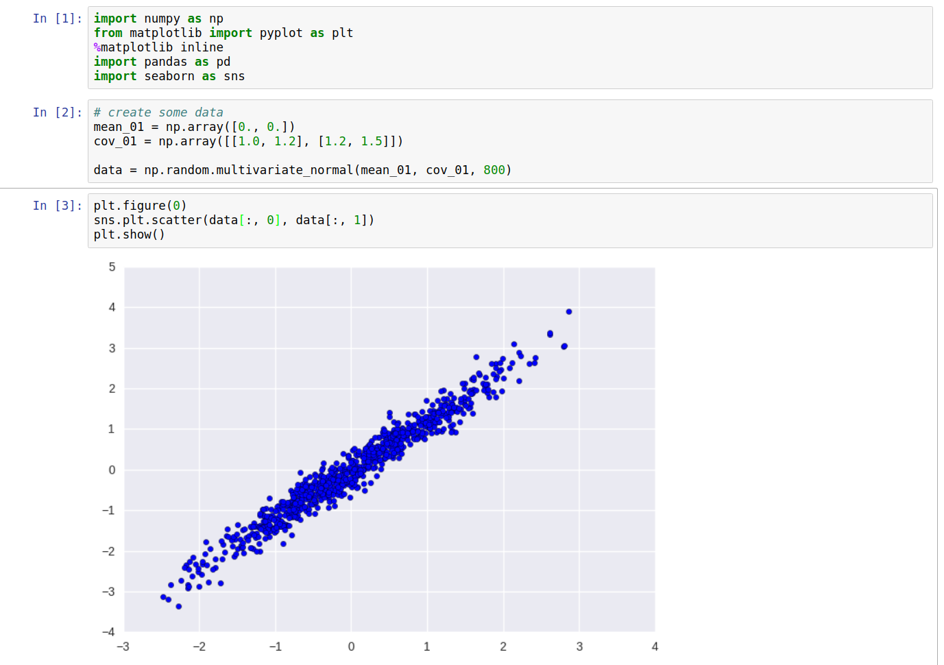
We want to figure out a transformation function \(W\) and apply on the data \(X\) so that in the resulting data \(Y\), the variables will be independent of each other. In simple terms, the covariance between any two distinct columns of \(Y\) will be zero, i.e. the non-diagonal elements of the covariance matrix \(C_Y\) of \(Y\) will be zero. This implies that \(C_Y\) will be a diagonal matrix.

Writing the transformation from \(X\) to \(Y\), we have:

To solve for the covariance matrix of Y, we can write

and since, \(Y = W\cdot X\), we have,

or,

We know that, \(C_Y\) is supposed to be a diagonal matrix. What does this equation remind us of? but of course, the Singular Value Decomposition (SVD). Thus, If we take \(W\) as the matrix of the eigenvectors and \(C_Y\) as the diagonal matrix of the eigenvalues, the above equation will hold true, making the matrix \(W\), of eigenvectors of covariance of \(X\), our transformation matrix.

Computing the above values for our data, and plotting the directions of the obtained eigenvalues, we get the following:

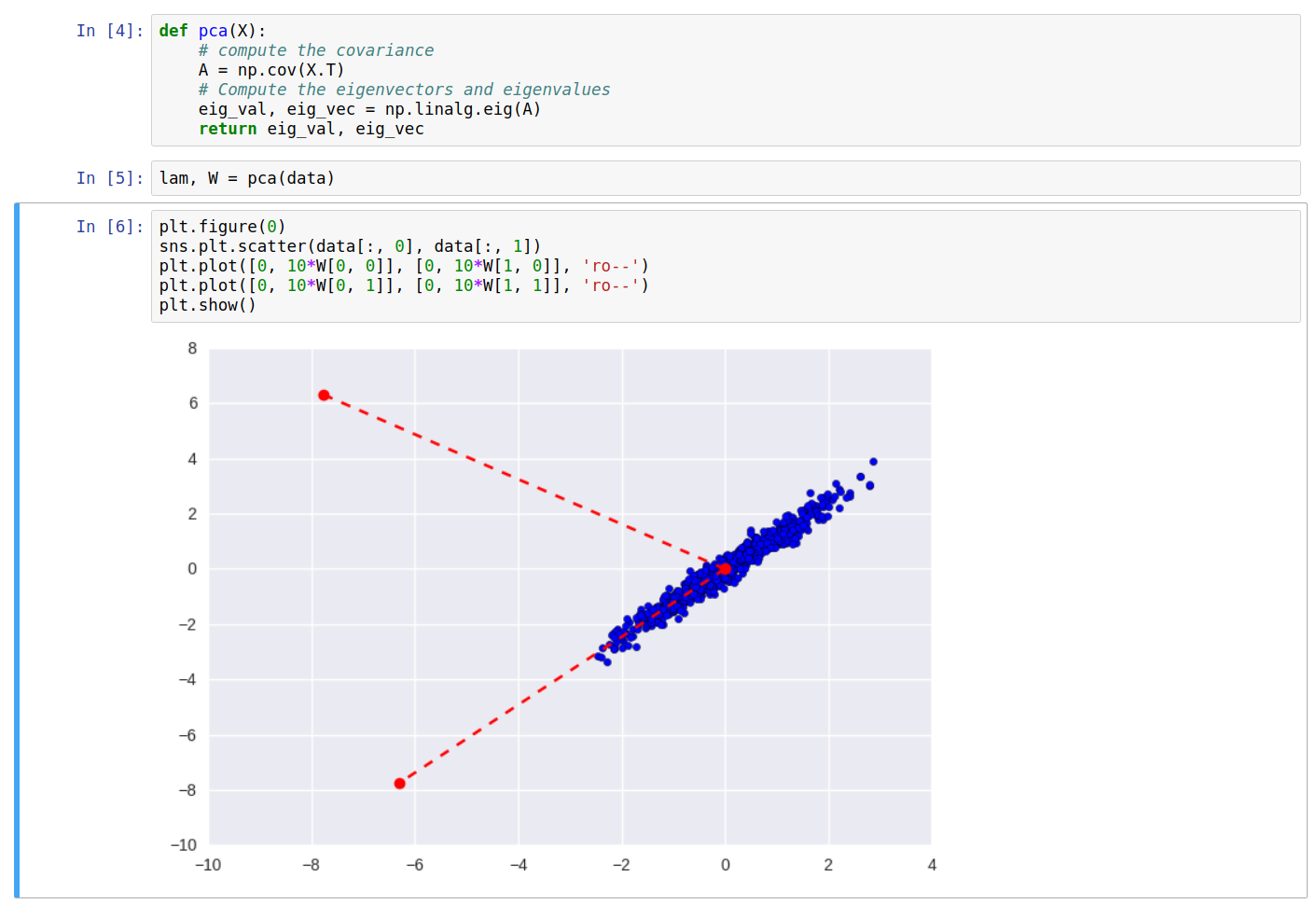
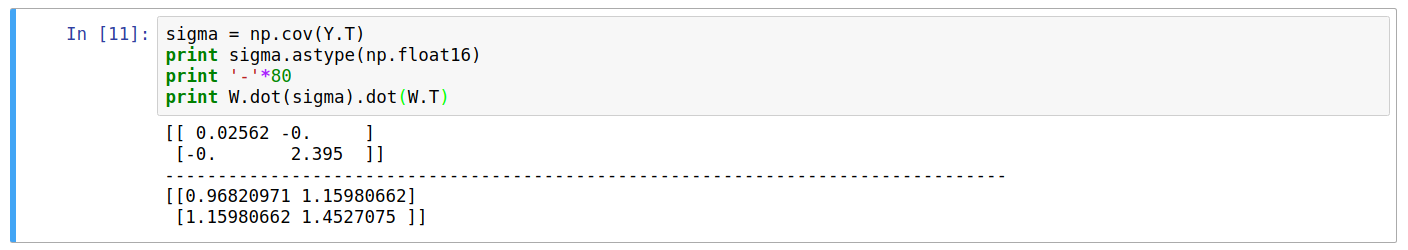
As can be seen clearly, one of the eigenvectors falls along the direction of maximum variance of the data. On transforming the data \(X\) into \(Y\), and plotting again, we get:

Printing the covariance of the new data \(Y\), we can see it’s a diagonal matrix. Also, the equation \(W\cdot C_Y\cdot W^T\) returns the original covariance matrix \(C_X\).

Dimension Reduction

One of the major applications of PCA is it’s ability to choose the dimensions of maximum variation, i.e. taking the projection of the data along those components only will not affect the complexity of the data by a significant amount and data can be reconstructed back to an approximation of it’s original form with the lower dimensional data as well.

On paying more attention to the covariance matrix \(C_Y\), we see that the magnitude of the eigenvalues along the diagonal of the matrix is related to the amount of variances explained by the said eigenvector direction.

So, sorting the eigenvalues and corresponding eigenvector pairs in decreasing order and taking only the top values becomes the ideal way of choosing the eigenvectors for obtaining maximum explained variances.

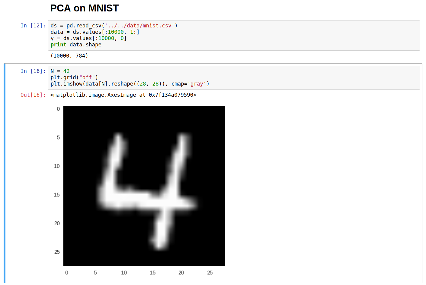
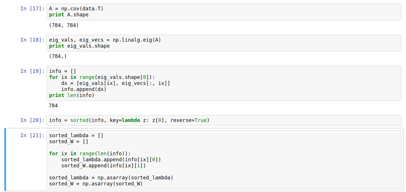
For further demonstration, let’s use another dataset (MNIST) for PCA.

Computing the eigenvectors and eigenvalues for the above dataset and sorting them on the basis of eigenvalues (descending order), we can store them back in numpy arrays.

And plot the eigenvalues, and the cumulative sum of the eigenvalues (Explained Variances).

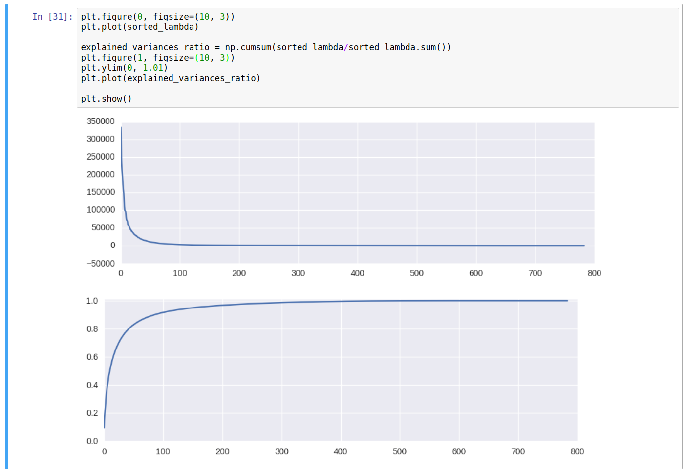
From the above curve for the cumulative sum, denoting the explained variances of the original data, we can conclude that approximate 150 dimensions shall be enough to get ~95% of the variances of the original dataset, and about 326 dimensions out of 784 for ~99%.

To reduce the number of dimensions, we have to select the number of dimensions we want \(k\) and use only those \(k\) columns from \(W\) to form the transformation matrix (Say \(W'\)). Thus the transformation and reconstruction operation become:

Let’s now pick only 2 dimensions (~23% explained variance), and plot the points as a scatter plot, and color based on the class label from the training set. Let’s use scikit-learn package for this last operation:

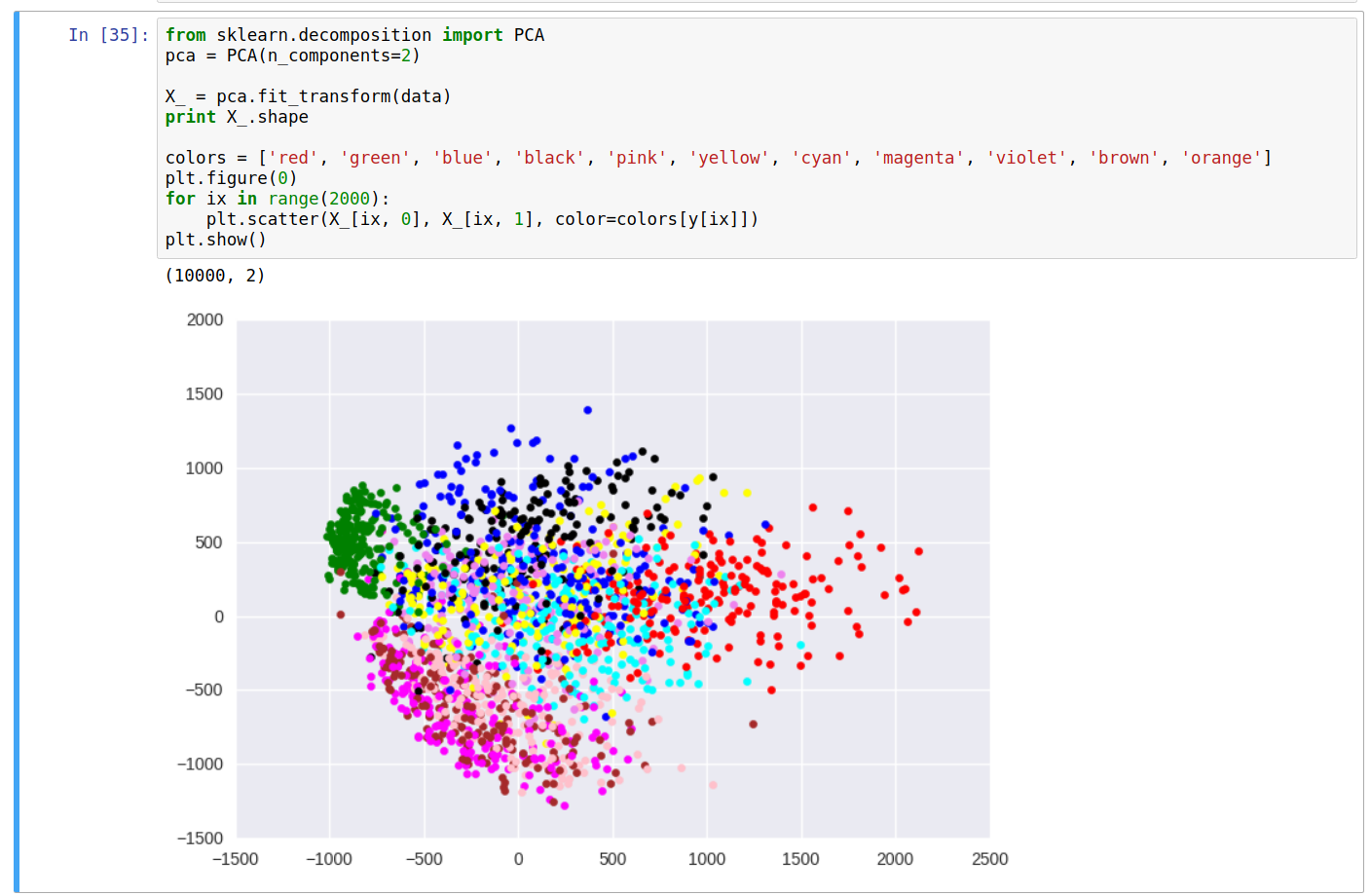
From the scatter plot, we can do some simple analysis and see some relationship between the color of points (labels) and their location on the plot. For instance, the green cluster (representing the label 1) is formed clearly distinct from others, while the clusters for colors brown and pink (for digits 4 and 9) are somewhat in the same region, etc.

Although the explained variance with 2 dimensions was roughly 23%, we still can derive some meaningful information about the data. Having more number of dimensions will make it easier to process and analyse the data as compared to the original data distribution.

Also, applying PCA would make it easier to use the data in models such as the Naive Bayes, where the core assumption is that the columns are independent of each other.

Note: If we want to keep the physical meaning of the columns in the dataset intact, using PCA would be a bad idea since the transformed columns are linear combinations of the original columns. Hence, the new columns would lose their original meaning.

Also, dimension reduction is useful only if the eigenvalues vary significantly for any data distribution. For eigenvalues in similar ranges, each column will have similar contribution towards the variation in data, hence removing them would cause greater loss.

–