Semi-Implicit Networks
Semi-Implicit Networks
Residual Neural Networks, or ResNets
The similarity of ResNet architecture with Ordinary Differential Equations has been under some attention in recent works
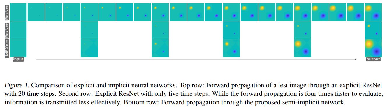
This post closely follows (read shamelessly copies) the work presented in IMEXnet - Forward Stable Deep Neural Network
In this post, I have discussed the concept of semi-implicit methods provided by the authors. For a detailed view and experimental analysis, head over to their paper
and their github repo
Residual Method as ODE
The $j^{th}$ layer of a Residual layer, updating the feature $Y_j$ can be written as:
\begin{equation} Y_{j+1} = Y_{j} + h.f(Y_{j}, \theta_{j}) \tag{1} \label{eq:one} \end{equation}
Where, $Y_{j+1}$ and $Y_j$ are outputs of layers $j+1$ and $j$ respectively. $\theta_j$ is the layer parameter, $f$ is a non-linear function, and $h$ is the step size (usually set to 1). In problems related to images, the function $f$ is usually a series of convolutions, normalisation and activations. In this particular work, $f$ is taken to be:
\begin{equation} f(Y, K_1, K_2, \alpha, \beta) = K_2 \sigma (N_{\alpha,\beta} (K_1 Y)) \tag{2} \label{eq:two} \end{equation}
Here $K_1$ and $K_2$ are taken to be 3x3 convolutional kernels, $N_{\alpha,\beta}$ is the normalization layer and $\sigma$ is the non-linear activation function. This structure was taken from
Forward Euler Form
In lieu of the step function described in \eqref{eq:one} (the discretized form), the forward euler formulation of the ODE is written as:
\begin{equation} \dot Y(t) = f(Y(t), \theta(t))
Y(0) = Y_0 \tag{3} \label{eq:three} \end{equation}
The features $Y(t)$ and the weights $\theta(t)$ are taken to be continuous functions in time, where $t$ corresponds to the depth of the network. Previously, explicit methods (such as mid-point method, Runge Kutta method) have been utilised to solve such equations, they often suffer from a lack of stability. Explicit methods are of the form where the information in $Y_{t+1}$ is described as a functoin of the previous state $Y_t$. Using some iterative methods (as mentioned in examples above), many small steps are usually needed to integrate the PDE over a long amount of time.
As mentioned in the paper, one way to improve the flow of information in the network modelled after ODEs is to make use of implicit methods, i.e. express the state $Y_{t+1}$ in terms of the same time-step $Y_{t+1}$ implicitly.
Semi-Implicit Form and It’s Stability
One of the simplest forms for implicit functions, quite similar to forward euler equation is the backward euler method in the non-linear discretized form:
\begin{equation} Y_{j+1} - Y_{j} = h . f(Y_{j+1}, \theta_{j+1}) \tag{4} \label{eq:four} \end{equation}
This method is stable for any choice of $h$ when the eigenvalue of the jacobian of $f$ have no positive real part (See This article for more details on stability of methods w.r.t to second-order differential equations). If the given condition is satisfied, $h$ can be chosen large enough to simulate large step-size in the continuous form while being robust to small perturbations in the input information.
Turns out, implicit methods are rather expensive to compute. Especially the above mentioned equation \eqref{eq:four} is a non-linear problem which can be computationally expensive to solve. So rather than using a full implicit or explicit method, the authors derived a combination in the form of a implicit-explicit (IMEX) or semi-implicit method.
They key idea in IMEX methods is to divide the right-hand side of the ODE into two parts: A non-linear explicit form and a linear implicit form. The equation in IMEXnet is designed in such a way that it can be solved efficiently. The equation in \eqref{eq:three} will now be reformatted as:
\begin{equation} \dot Y(t) = f(Y(t), \theta(t)) + LY(t) - LY(t) \tag{5} \label{eq:five} \end{equation}
where, The first part $f(Y(t), \theta(t)) + LY(t)$ is treated explicitly, while the second part $LY(t)$ is treated implicitly.
The matrix $L$ is chosen freely with the property of being easily invertible. A fair choice of $L$ can be modelled after a 3x3 convolution operation with symmetric positive-definite property, which makes it easy to invert (more on that later). The continuous equation can now be simplified as the following:
which can be simplified as:
\begin{equation} Y_{j+1} = (I - hL)^{-1} (Y_j + hLY_j + hf(Y_j, \theta_j)) \tag{6} \label{eq:six} \end{equation}
with $I$ being the identity matrix.
In the above equation, the authors have shown that the forward part (while seemingly complex) is rather easy to compute and similar to that of a convolution. Furthermore, the authors claim that the network is always stable for a suitable choice of $L$, while having some favourable properties of implicit methods. The matrix $(I + hL)^{-1}$ is dense in nature, which avoids the field of view problem by using all pixels of the image in it’s computational step.
The authors choose $L$ to be a laplacian matrix with a group convolution operator (group conv. was also used in AlexNet!
Before going into the discussion about the choice of $L$ and the stability of the method, a quick recap of the Laplace transform is due.
The [Laplace transform](https://en.wikipedia.org/wiki/Laplace_transform) (taken from wikipedia), converts a function of real variable $t$ to a function of a complex variable $s$. The laplace transform for $f(t); t \ge 0$ is the function $F(s)$ which is a unilteral transform defined by: $$ F(s) = \int_{0}^{\infty} f(t) e^{-st} dt $$ And, for a laplacian matrix, $L$ is defined as, $L = D - A$ for a graph $G$, where $A$ is the adjacency matrix and $D$ is the degree matrix of the graph $G$.
Now, on the stability of the method, the authors provide a wonderful example of a simplified setting with a model problem (as given below) and provide the reasoning for the aforementioned choice of $L$.
\begin{equation} \dot Y(t) = \lambda Y(t)
Y(t) = Y_0 \tag{8} \end{equation}
And take $L = \alpha I$, where we choose $\alpha \ge 0$. (Refer to the paper for a complete proof). Based on the analysis, the authors choose $K_1 = -K_{2}^{\intercal}$ in the equation \eqref{eq:two} as discussed properly in
An example of the field of view is shown here for IMEXnet.
The Forward Pass
The authors show that using already available and widely used tools such as auto-differentiation and the fast fourier transform (FFT), an efficient way for computing the linear system given below can be found.
\[(I + hL)Y = B\]where, $L$ is constructed like a group-wise convolution as mentioned earlier and $B$ collects the explicit term.
For efficient solution to the system, authors make use of the convolution theorem in the fourier space. The theorem says, for a convolution operation between a kernel $A$ and features $Y$, the convolutional operation can be computed as:
\begin{equation} A * Y = F^{-1}((FA) \odot (FY)) \tag{9} \label{eq:nine} \end{equation}
Where, $F$ is the Fourier transform, $*$ is the convolution operator, and $\odot$ is the hadamard-product (element-wise multiplication). Here, we assume a periodic boundary on the image data (discussed in detail next). This implies that if we need to compute the product of inverse of the convolutional operator $A$, we can simply element-wise divide by the inverse fourier transform of $A$:
\[A^{-1} * Y = F^{-1}((FY) \oslash (FA))\]In our case, the kernel $A$ is associated with the matrix $I + hL$, which is invertible. For example, when we choose $L$ to be positive semi-definite, we define:
\[L = B^{\intercal} B\]Where, $B$ is a trainable group-convolution operator. Using Fourier methods, we need to have the convolutional kernel at the same size as the image we convolve it with. This is done by generating a zero-matrix as the same size as that of the image and inserting entries of the kernel at appropriate places.
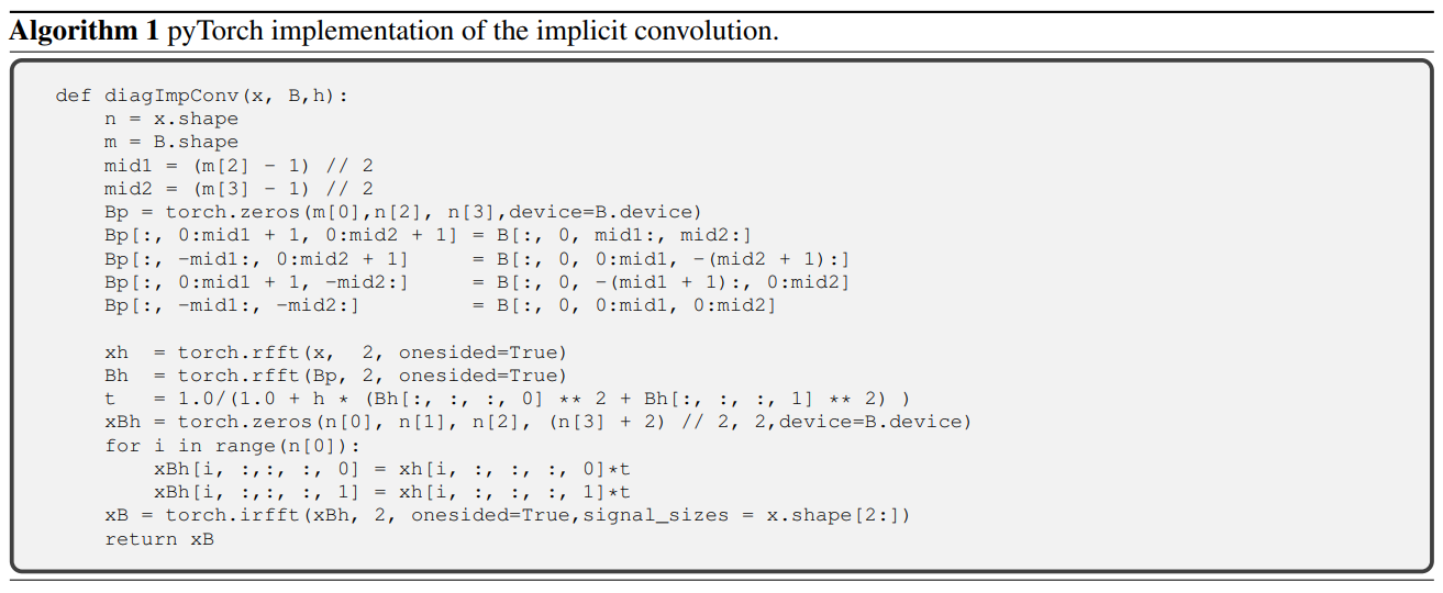
For a more thorough explaination about how to construct this kernel for fourier method, refer to the book. The periodic boundary condition and the positive semi-definite property of the kernel are important here to derive the final convolution kernel $A$ for fourier transform and it’s spectral decomposition. Specifically, in chapters 3 and 4 of the book, it is given in detail about how to form the convolution kernel (or toeplitz matrix) for the __BCCB (Boundary Circulant with Circulat Blocks)__ type matrix. All BCCB matrices are normal in nature, i.e. $A^{*} A = A A^{*}$. So, a basic outline to compute the equation \eqref{eq:nine} is: Refer to
- Compute the center of the kernel (after zero padding to match the size)
- Apply the corresponding circular shift over the kernel with the center.
- Compute the fourier transform of the update kernel and the image.
- Take the inverse fourier transform of the product.
for a detailed information about the process, and [convolution theorem](https://en.wikipedia.org/wiki/Convolution_theorem)</a> for a proof of the equation \eqref{eq:nine}.
The method is wonderfully captured by the authors with the help of a PyTorch pseudo-code as following:
Computational Complexity
For a single block ResNet, with m channels and input image of size sxs, the forward pass takes approximately $\mathcal{O}(m^2 s^2)$ operations and $\mathcal{O}(m^2)$ memory.
For the IMEX network, the explicit is pretty much the same followed by the implicit step. The Implicit step is a group-wise convolutional operation and requires $\mathcal{O}(m(s.log(s))^2)$ additional operations. The $s.log(s)$ term results from the application of the fourier transform. Since $log(s)$ is typically much smaller than $m$, the additional cost can be considered insignificant.
Final Notes
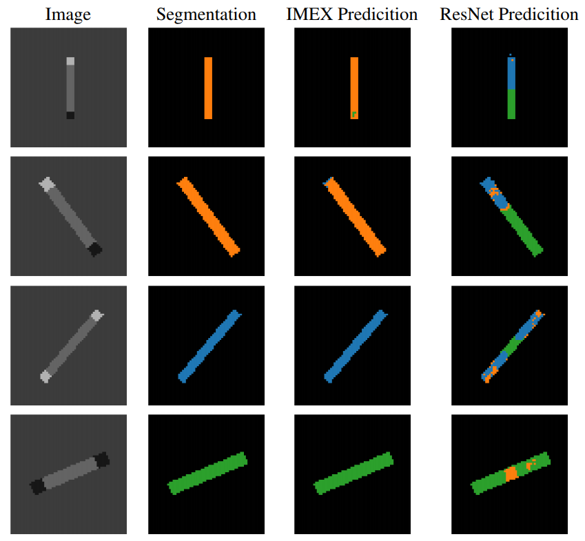
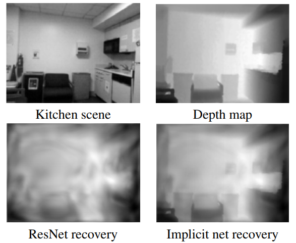
As for the effectiveness of the network, the authors provide some compelling results on problems such as segmentation on synthetic Q-tip images as a toy example, and depth-estimation over kitchen images from the NYU Depth V2
First example from the Qtip segmentation:
And an example from the depth estimation for kitchen images taken from the NYU Depth V2 dataset
The authors also make note of further possibilities for choosing other models with similar implicit properties. They epecially make note of a variant that can be used (called the diffusion-reaction problem):
\[\dot Y(t) = f(Y(t), \theta(t)) - LY(t)\]Such equations can have interesting behaviour like forming non-linear wave patterns etc. These systems have been already studied in rigourous details as mentioned in the paper.
Some further work over this appproach is also discussed in the paper: Robust Learning with Implicit Residual Networks
NOTE: I have written this post as per my understanding of the paper, and for my learning. I have tried to summarize (mostly just copy) the paper to the best of my capability in a short duration. Any constructive reviews are welcome.
–